Magika: AI powered fast and efficient file type identification

Today we are open-sourcing Magika, Google’s AI-powered file-type identification system, to help others accurately detect binary and textual file types. Under the hood, Magika employs a custom, highly optimized deep-learning model, enabling precise file identification within milliseconds, even when running on a CPU.

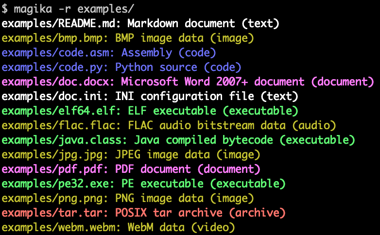
Magika command line tool used to identify the type of a diverse set of files

You can try the Magika web demo today, or install it as a Python library and standalone command line tool (output is showcased above) by using the standard command line pip install magika.

Why identifying file type is difficult

Since the early days of computing, accurately detecting file types has been crucial in determining how to process files. Linux comes equipped with libmagic and the file utility, which have served as the de facto standard for file type identification for over 50 years. Today web browsers, code editors, and countless other software rely on file-type detection to decide how to properly render a file. For example, modern code editors use file-type detection to choose which syntax coloring scheme to use as the developer starts typing in a new file.

Accurate file-type detection is a notoriously difficult problem because each file format has a different structure, or no structure at all. This is particularly challenging for textual formats and programming languages as they have very similar constructs. So far, libmagic and most other file-type-identification software have been relying on a handcrafted collection of heuristics and custom rules to detect each file format.

This manual approach is both time consuming and error prone as it is hard for humans to create generalized rules by hand. In particular for security applications, creating dependable detection is especially challenging as attackers are constantly attempting to confuse detection with adversarially-crafted payloads.

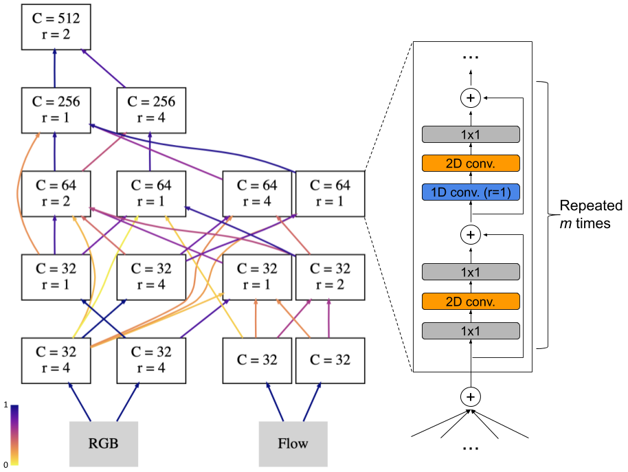
To address this issue and provide fast and accurate file-type detection we researched and developed Magika, a new AI powered file type detector. Under the hood, Magika uses a custom, highly optimized deep-learning model designed and trained using Keras that only weighs about 1MB. At inference time Magika uses Onnx as an inference engine to ensure files are identified in a matter of milliseconds, almost as fast as a non-AI tool even on CPU.

Magika Performance

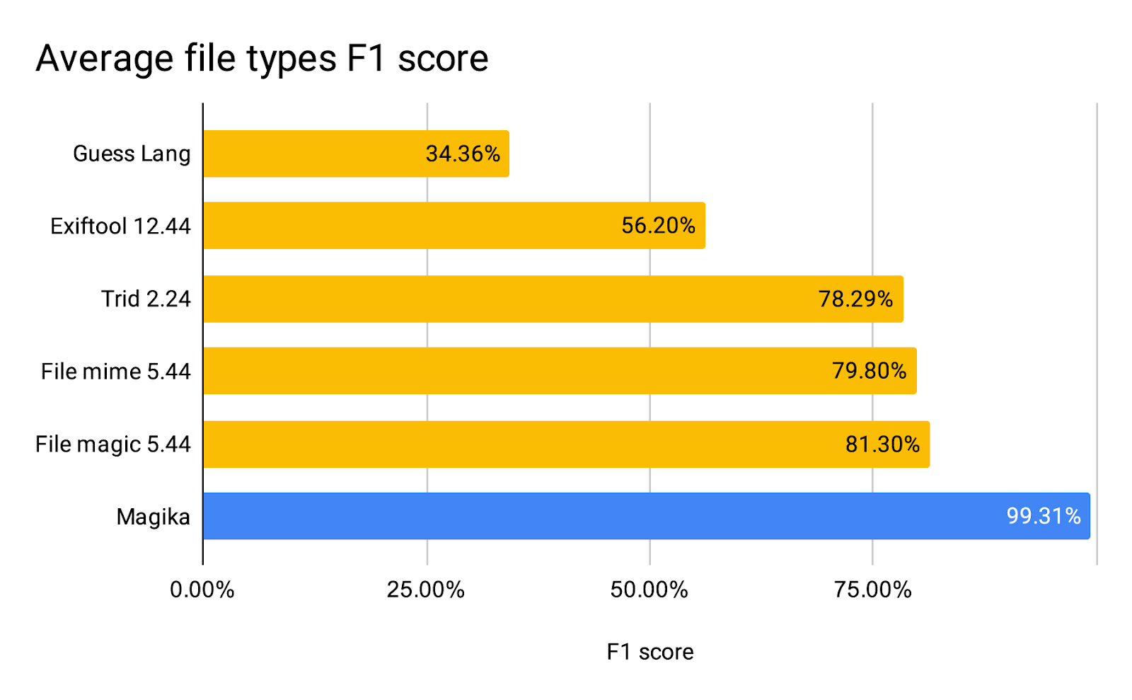
Magika detection quality compared to other tools on our 1M files benchmark

Performance wise, Magika, thanks to its AI model and large training dataset, is able to outperform other existing tools by about 20% when evaluated on a 1M files benchmark that encompasses over 100 file types. Breaking down by file type, as reported in the table below, we see even greater performance gains on textual files, including code files and configuration files that other tools can struggle with.

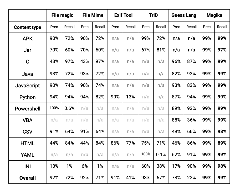
Various file type identification tools performance for a selection of the file types included in our benchmark - n/a indicates the tool doesn’t detect the given file type.

Magika at Google

Internally, Magika is used at scale to help improve Google users’ safety by routing Gmail, Drive, and Safe Browsing files to the proper security and content policy scanners. Looking at a weekly average of hundreds of billions of files reveals that Magika improves file type identification accuracy by 50% compared to our previous system that relied on handcrafted rules. In particular, this increase in accuracy allows us to scan 11% more files with our specialized malicious AI document scanners and reduce the number of unidentified files to 3%.

The upcoming integration of Magika with VirusTotal will complement the platform's existing Code Insight functionality, which employs Google's generative AI to analyze and detect malicious code. Magika will act as a pre-filter before files are analyzed by Code Insight, improving the platform’s efficiency and accuracy. This integration, due to VirusTotal’s collaborative nature, directly contributes to the global cybersecurity ecosystem, fostering a safer digital environment.

Open Sourcing Magika

By open-sourcing Magika, we aim to help other software improve their file identification accuracy and offer researchers a reliable method for identifying file types at scale.

Magika code and model are freely available starting today in Github under the Apache2 License. Magika can also quickly be installed as a standalone utility and python library via the pypi package manager by simply typing pip install magika with no GPU required. We also have an experimental npm package if you would like to use the TFJS version.

To learn more about how to use it, please refer to Magika documentation site.

Acknowledgements

Magika would not have been possible without the help of many people including: Ange Albertini, Loua Farah, Francois Galilee, Giancarlo Metitieri, Luca Invernizzi, Young Maeng, Alex Petit-Bianco, David Tao, Kurt Thomas, Amanda Walker, and Zhixun Tan.

By Elie Bursztein – Cybersecurity AI Technical and Research Lead and Yanick Fratantonio – Cybersecurity Research Scientist

DeepNull: an open-source method to improve the discovery power of genetic association studies

In our paper “DeepNull models non-linear covariate effects to improve phenotypic prediction and association power,” we proposed a new method, DeepNull, to model the complex relationship between covariate effects on phenotypes to improve Genome-wide association studies (GWAS) results. We have released DeepNull as open source software, with a Colab notebook tutorial for its use.

Human Genetics 101

Each individual’s genetic data carries health information such as why certain individuals have a lower risk of developing skin cancer compared to others or why certain drugs differ in effectiveness between individuals. Genetic data is encoded in the human genome—a DNA sequence—composed of a 3 billion long chain built from four possible nucleotides (A, C, G, and T). Only a small subset of the genome (~4-5 million positions) varies between two individuals. One of the goals of genetic studies is to detect variants that are associated with different phenotypes (e.g., risk of diseases such as Glaucoma or observed phenotypic values such as high-density lipoprotein (HDL), low-density lipoproteins (LDL), height, etc).

Genome-wide association studies

GWAS are used to associate genetic variants with complex traits and diseases. To more accurately determine an association strength between genotype and phenotype, the interactions between phenotypes (such as age and sex) and principal components (PCs) of genotypes, must be adjusted for as covariates. Covariate adjustment in GWAS can increase precision and correct for confounding. In the linear model setting, adjustment for a covariate will improve precision (i.e., statistical power) if the distribution of the phenotype differs across levels of the covariate. For example, when performing GWAS on height, males and females have different means. All state of the art methods (e.g., BOLT-LMM, regenie) perform GWAS assuming that the effect of genotypes and covariates to phenotype is linear and additive. However, we know that the assumption of linear and additive contributions of covariates often does not reflect underlying biology, so we sought a method to more comprehensively model and adjust for the interactions between phenotypes for GWAS.

DeepNull method overview

We proposed a new method, DeepNull, to relax the linear assumption of covariate effects on phenotypes. DeepNull trains a deep neural network (DNN) to predict phenotype using all covariates in a 5-fold cross-validation. After training the DeepNull model, we make phenotype predictions for all individuals and add this prediction as one additional covariate in the association test. Major advantages of DeepNull are its simplicity to use and that it requires only a minimal change to existing GWAS pipeline implementations. In other words, to use DeepNull, we just need to add one additional covariate, which is computed by DeepNull, to the existing pipeline to perform GWAS.

DeepNull improves statistical power

We simulated data under different genetic architectures (genetic conditions) to first check that DeepNull controls type I error and then compare DeepNull statistical power with current state of the art methods (hereafter referred to as “Baseline”). First, we simulated data under genetic architectures where covariates have a linear effect on phenotype and observed that both Baseline and DeepNull have tight control of type I error. It is interesting that DeepNull power does not decrease compared to Baseline under a setting in which covariates have only a linear effect on phenotype. Next, we simulated data under genetic architectures where covariates have non-linear effects on phenotype. Both Baseline and DeepNull have tight control of type I error while DeepNull increases the statistical power depending on the genetic architecture. We observed that for certain genetic architectures, DeepNull increases the statistical power up to 20%. Below, we compare the -log p-value of test statistics computed from DeepNull versus Baseline for Apolipoprotein B (ApoB) levels obtained from UK Biobank:

Figure 1. Significance level comparison of DeepNull vs Baseline. X-axis is the -log p-value of Baseline and Y-axis is the -log p-value of DeepNull. The orange dots indicate variants that are significant for Baseline but not significant for DeepNull and green dots indicate variants that are significant for DeepNull but not significant for Baseline.

DeepNull improves phenotype prediction

We applied DeepNull to predict phenotypes by utilizing polygenic risk score (PRS) and existing covariates such as age and sex. We considered 10 phenotypes obtained from UK Biobank. We observed that DeepNull on average increased the phenotype prediction (R2 where R is Pearson correlation) by 23%. More strikingly, in the case of Glaucoma, referral probability that is computed from the fundus images (Phene et al. Ophthalmology 2019, Alipanahi et al AJHG 2021), DeepNull improves the phenotype prediction by 83.4% and in the case of LDL, DeepNull improves the phenotype prediction by 40.3%. The summary of DeepNull results versus Baseline are shown in figure 2 below:

 

 

Figure 2. DeepNull improves phenotype prediction compared to Baseline. The Y-axis is the R2 where R is the Pearson’s correlation between true and predicted value of phenotypes. Phenotypic abbreviations: alkaline phosphatase (ALP), alanine aminotransferase (ALT), aspartate aminotransferase (AST), apolipoprotein B (ApoB), glaucoma referral probability (GRP), LDLcholesterol (LDL), sex hormone-binding globulin (SHBG), and triglycerides (TG).

Conclusion

We proposed a new framework, DeepNull, that can model the nonlinear effect of covariates on phenotypes when such nonlinearity exists. We show that DeepNull can substantially improve phenotype prediction. In addition, we show that DeepNull achieves results similar to a standard GWAS when the effect of covariate on the phenotype is linear and can significantly outperform a standard GWAS when the covariate effects are nonlinear. DeepNull is open source and is available for download from GitHub or installation via PyPI.

By Farhad Hormozdiari and Andrew Carroll – Genomics team in HealthAI

Acknowledgments

This blog summarizes the work of the following Google contributors, who we would like to thank: Zachary R. McCaw, Thomas Colthurst, Ted Yun, Nick Furlotte, Babak Alipanahi, and Cory Y. McLean. In addition, we would like to thank Alkes Price, Babak Behsaz, and Justin Cosentino for their invaluable comments and suggestions.

Analyzing genomic data in families with deep learning

The Genomics team at Google Health is excited to share our latest expansion to DeepVariant - DeepTrio.

First released in 2017, DeepVariant is an open source tool that enables researchers and clinicians to analyze an individual’s genome sequencing data and identify genetic variants, such as those that may cause disease. Our continued work on DeepVariant has been recognized for its top-of-class accuracy. With DeepTrio, we have expanded DeepVariant to be able to consider the genetic variants in the sequence data of a mother-father-child trio.

Humans are diploid organisms, carrying two copies of the human genome. Every individual inherits one copy of the genome from their mother, and the other from their father. Parental inheritance informs analysis of traits and diseases that follow Mendelian inheritance. DeepTrio learns to use the properties of Mendelian inheritance directly from sequencing data in order to more accurately identify genetic variants in cases when both parent and a child sample can be co-analyzed.

Modifying DeepVariant to analyze trio samples

DeepVariant learns to classify positions in a genome as reference or variant using representations of data similar to the “genome browser” which experts use in analysis. “Improving the Accuracy of Genomic Analysis with DeepVariant 1.0” provides a good overview.

DeepVariant receives data as a window of the genome centered on a candidate variant which it is asked to classify as either reference (no variant), heterozygous (one copy of a variant) or homozygous (both copies are variant). DeepVariant sees the sequence evidence as channels representing features of the data (see: “Looking through DeepVariant’s eyes” for a deeper explanation).

We modified DeepTrio to represent the sequence data from a trio in a single image, with a fixed height for each sample and the child in the middle. Using gold standard samples from NIST Genome in a Bottle for truth labels, we train one model to call variants in the child and another to call variants in the top parent. To call both parents, we flip the position of the parent samples.

Figure 1. (top) An image of 4 of the channels that DeepTrio uses in classification (these, and 4 other channels are shown in a stack. (bottom) conceptual schematic of how trio files are used to create examples, which are then called by DeepTrio.

Measuring DeepTrio’s improved accuracy

We show that DeepTrio is more accurate than DeepVariant for both parent and child variant detection, with an especially pronounced advantage at lower coverages. This enables researchers to either analyze samples at higher accuracy, or to maintain comparable accuracy at a substantially reduced expense.

To assess the accuracy of DeepTrio, we compare its accuracy to DeepVariant using extensively characterized gold standards made available by NIST Genome in a Bottle. In order to have an evaluation dataset which is never seen in training, we exclude chromosome 20 from training and perform evaluations on chromosome 20.

We train DeepVariant and DeepTrio for sequencing data from two different instruments, Illumina and Pacific Biosciences (PacBio), for more information on the differences between these technologies, please see our previous blog. These sequencers both randomly sample the genome in an error-prone manner. To accurately analyze a genome, the same region needs to be sampled repeatedly. The depth of sampling at a position is called coverage. Sequencing to greater coverage is more expensive in an approximately linear manner. This often forces trade-offs between cost, accuracy, and samples sequenced. As a result, in trios parents are often sequenced at lower depth.

In the charts below, we plot the accuracy of DeepTrio and DeepVariant across a range of coverages.

Figure 2. F1-score for DeepTrio (solid line) and DeepVariant (dashed line) on a child sample (top) and a parent sample (bottom), sequenced with an Illumina (blue) and PacBio (black) instrument. F1 is measured for all types of small variants on chromosome 20, across samples with a range of sequencing coverage (x-axis).

DeepTrio’s performance on de novo variants

Each individual has roughly 5 million variants relative to the human reference genome. The overwhelming majority of these are inherited from their parents. A small number, around 100, are new (referred to as de novo), due to copying errors during DNA replication. We demonstrate that DeepTrio substantially reduces false positives for de novo variants. For Illumina data, this comes with a smaller decrease in recovery of true positives, while for PacBio data, this trade-off does not occur.

To assess accuracy we analyzed sites where both parents are called as non-variant, but the child is called as heterozygous variant. We observe that DeepTrio is more reluctant to call a variant as de novo, which is similar to how a human would require a higher level of evidence for sites violating Mendelian inheritance. This results in a much lower false positive rate for these de novo variants, but a slightly lower recall rate in DeepTrio Illumina. Usually when this occurs, the child is still called as a variant, but the parents are given “no-call” (the classifier is not confident enough to make a call).

Figure 3. Accuracy on de novo calls (child heterozygous variant, parents reference call) for recall of true de novo events (top) and false positive de novo events (bottom) for DeepTrio (solid line) and DeepVariant (dashed line) on Illumina (blue) and PacBio (black). Accuracy is measured on chromosome 20, across samples with a range of sequencing coverage (x-axis).

Contributing to rare disease research

By releasing DeepTrio as open source software, we hope to improve analysis of genomic data, by allowing scientists to more accurately analyze samples. We hope this will enable research and clinical pipelines, leading to better resolution of rare disease cases, and improve development of therapeutics.

In addition to the release of DeepTrio’s code as open source, we have also released the sequencing data that we generated in order to train these models. That data is described in our pre-print “An Extensive Sequence Dataset of Gold-Standard Samples for Benchmarking and Development”. By releasing both this production model, and the data required to train models of similar complexity, we hope to contribute to methods development by the genomics community.

By Andrew Carroll, Product Lead Genomics and Howard Yang, Program Manager Genomics — Google Health

AutoFlip: An Open Source Framework for Intelligent Video Reframing

Originally posted on the AI Blog

Videos filmed and edited for television and desktop are typically created and viewed in landscape aspect ratios (16:9 or 4:3). However, with an increasing number of users creating and consuming content on mobile devices, historical aspect ratios don’t always fit the display being used for viewing. Traditional approaches for reframing video to different aspect ratios usually involve static cropping, i.e., specifying a camera viewport, then cropping visual contents that are outside. Unfortunately, these static cropping approaches often lead to unsatisfactory results due to the variety of composition and camera motion styles. More bespoke approaches, however, typically require video curators to manually identify salient contents on each frame, track their transitions from frame-to-frame, and adjust crop regions accordingly throughout the video. This process is often tedious, time-consuming, and error-prone.

To address this problem, we are happy to announce AutoFlip, an open source framework for intelligent video reframing. AutoFlip is built on top of the MediaPipe framework that enables the development of pipelines for processing time-series multimodal data. Taking a video (casually shot or professionally edited) and a target dimension (landscape, square, portrait, etc.) as inputs, AutoFlip analyzes the video content, develops optimal tracking and cropping strategies, and produces an output video with the same duration in the desired aspect ratio.

Left: Original video (16:9). Middle: Reframed using a standard central crop (9:16). Right: Reframed with AutoFlip (9:16). By detecting the subjects of interest, AutoFlip is able to avoid cropping off important visual content.

AutoFlip Overview

AutoFlip provides a fully automatic solution to smart video reframing, making use of state-of-the-art ML-enabled object detection and tracking technologies to intelligently understand video content. AutoFlip detects changes in the composition that signify scene changes in order to isolate scenes for processing. Within each shot, video analysis is used to identify salient content before the scene is reframed by selecting a camera mode and path optimized for the contents.

Shot (Scene) Detection

A scene or shot is a continuous sequence of video without cuts (or jumps). To detect the occurrence of a shot change, AutoFlip computes the color histogram of each frame and compares this with prior frames. If the distribution of frame colors changes at a different rate than a sliding historical window, a shot change is signaled. AutoFlip buffers the video until the scene is complete before making reframing decisions, in order to optimize the reframing for the entire scene.

Video Content Analysis

We utilize deep learning-based object detection models to find interesting, salient content in the frame. This content typically includes people and animals, but other elements may be identified, depending on the application, including text overlays and logos for commercials, or motion and ball detection for sports.

The face and object detection models are integrated into AutoFlip through MediaPipe, which uses TensorFlow Lite on CPU. This structure allows AutoFlip to be extensible, so developers may conveniently add new detection algorithms for different use cases and video content. Each object type is associated with a weight value, which defines its relative importance — the higher the weight, the more influence the feature will have when computing the camera path.

Left: People detection on sports footage. Right: Two face boxes (‘core’ and ‘all’ face landmarks). In narrow portrait crop cases, often only the core landmark box can fit.

Reframing

After identifying the subjects of interest on each frame, logical decisions about how to reframe the content for a new view can be made. AutoFlip automatically chooses an optimal reframing strategy — stationary, panning or tracking — depending on the way objects behave during the scene (e.g., moving around or stationary). In stationary mode, the reframed camera viewport is fixed in a position where important content can be viewed throughout the majority of the scene. This mode can effectively mimic professional cinematography in which a camera is mounted on a stationary tripod or where post-processing stabilization is applied. In other cases, it is best to pan the camera, moving the viewport at a constant velocity. The tracking mode provides continuous and steady tracking of interesting objects as they move around within the frame.

Based on which of these three reframing strategies the algorithm selects, AutoFlip then determines an optimal cropping window for each frame, while best preserving the content of interest. While the bounding boxes track the objects of focus in the scene, they typically exhibit considerable jitter from frame-to-frame and, consequently, are not sufficient to define the cropping window. Instead, we adjust the viewport on each frame through the process of Euclidean-norm optimization, in which we minimize the residuals between a smooth (low-degree polynomial) camera path and the bounding boxes.

Top: Camera paths resulting from following the bounding boxes from frame-to-frame. Bottom: Final smoothed camera paths generated using Euclidean-norm path formation. Left: Scene in which objects are moving around, requiring a tracking camera path. Right: Scene where objects stay close to the same position; a stationary camera covers the content for the full duration of the scene.

AutoFlip’s configuration graph provides settings for either best-effort or required reframing. If it becomes infeasible to cover all the required regions (for example, when they are too spread out on the frame), the pipeline will automatically switch to a less aggressive strategy by applying a letterbox effect, padding the image to fill the frame. For cases where the background is detected as being a solid color, this color is used to create seamless padding; otherwise a blurred version of the original frame is used.

AutoFlip Use Cases

We are excited to release this tool directly to developers and filmmakers, reducing the barriers to their design creativity and reach through the automation of video editing. The ability to adapt any video format to various aspect ratios is becoming increasingly important as the diversity of devices for video content consumption continues to rapidly increase. Whether your use case is portrait to landscape, landscape to portrait, or even small adjustments like 4:3 to 16:9, AutoFlip provides a solution for intelligent, automated and adaptive video reframing.

What’s Next?

Like any machine learning algorithm, AutoFlip can benefit from an improved ability to detect objects relevant to the intent of the video, such as speaker detection for interviews or animated face detection on cartoons. Additionally, a common issue arises when input video has important overlays on the edges of the screen (such as text or logos) as they will often be cropped from the view. By combining text/logo detection and image inpainting technology, we hope that future versions of AutoFlip can reposition foreground objects to better fit the new aspect ratios. Lastly, in situations where padding is required, deep uncrop technology could provide improved ability to expand beyond the original viewable area.

While we work to improve AutoFlip internally at Google, we encourage contributions from developers and filmmakers in the open source communities.

Acknowledgments

We would like to thank our colleagues who contributed to Autoflip, Alexander Panagopoulos, Jenny Jin, Brian Mulford, Yuan Zhang, Alex Chen, Xue Yang, Mickey Wang, Justin Parra, Hartwig Adam, Jingbin Wang, and Weilong Yang; MediaPipe team who helped with open sourcing, Jiuqiang Tang, Tyler Mullen, Mogan Shieh, Ming Guang Yong, and Chuo-Ling Chang.

By Nathan Frey, Senior Software Engineer, Google Research, Los Angeles and Zheng Sun, Senior Software Engineer, Google Research, Mountain View

Video Architecture Search

Video understanding is a challenging problem. Because a video contains spatio-temporal data, its feature representation is required to abstract both appearance and motion information. This is not only essential for automated understanding of the semantic content of videos, such as web-video classification or sport activity recognition, but is also crucial for robot perception and learning. Just like humans, an input from a robot’s camera is seldom a static snapshot of the world, but takes the form of a continuous video.

The abilities of today’s deep learning models are greatly dependent on their neural architectures. Convolutional neural networks (CNNs) for videos are normally built by manually extending known 2D architectures such as Inception and ResNet to 3D or by carefully designing two-stream CNN architectures that fuse together both appearance and motion information. However, designing an optimal video architecture to best take advantage of spatio-temporal information in videos still remains an open problem. Although neural architecture search (e.g., Zoph et al, Real et al) to discover good architectures has been widely explored for images, machine-optimized neural architectures for videos have not yet been developed. Video CNNs are typically computation- and memory-intensive, and designing an approach to efficiently search for them while capturing their unique properties has been difficult.

In response to these challenges, we have conducted a series of studies into automatic searches for more optimal network architectures for video understanding. We showcase three different neural architecture evolution algorithms: learning layers and their module configuration (EvaNet); learning multi-stream connectivity (AssembleNet); and building computationally efficient and compact networks (TinyVideoNet). The video architectures we developed outperform existing hand-made models on multiple public datasets by a significant margin, and demonstrate a 10x~100x improvement in network runtime.

EvaNet: The First Evolved Video Architectures

EvaNet, which we introduce in “Evolving Space-Time Neural Architectures for Videos” at ICCV 2019, is the very first attempt to design neural architecture search for video architectures. EvaNet is a module-level architecture search that focuses on finding types of spatio-temporal convolutional layers as well as their optimal sequential or parallel configurations. An evolutionary algorithm with mutation operators is used for the search, iteratively updating a population of architectures. This allows for parallel and more efficient exploration of the search space, which is necessary for video architecture search to consider diverse spatio-temporal layers and their combinations. EvaNet evolves multiple modules (at different locations within the network) to generate different architectures.

Our experimental results confirm the benefits of such video CNN architectures obtained by evolving heterogeneous modules. The approach often finds that non-trivial modules composed of multiple parallel layers are most effective as they are faster and exhibit superior performance to hand-designed modules. Another interesting aspect is that we obtain a number of similarly well-performing, but diverse architectures as a result of the evolution, without extra computation. Forming an ensemble with them further improves performance. Due to their parallel nature, even an ensemble of models is computationally more efficient than the other standard video networks, such as (2+1)D ResNet. We have open sourced the code.

Examples of various EvaNet architectures. Each colored box (large or small) represents a layer with the color of the box indicating its type: 3D conv. (blue), (2+1)D conv. (orange), iTGM (green), max pooling (grey), averaging (purple), and 1x1 conv. (pink). Layers are often grouped to form modules (large boxes). Digits within each box indicate the filter size.

AssembleNet: Building Stronger and Better (Multi-stream) models

In “AssembleNet: Searching for Multi-Stream Neural Connectivity in Video Architectures”, we look into a new method of fusing different sub-networks with different input modalities (e.g., RGB and optical flow) and temporal resolutions. AssembleNet is a “family” of learnable architectures that provide a generic approach to learn the “connectivity” among feature representations across input modalities, while being optimized for the target task. We introduce a general formulation that allows representation of various forms of multi-stream CNNs as directed graphs, coupled with an efficient evolutionary algorithm to explore the high-level network connectivity. The objective is to learn better feature representations across appearance and motion visual clues in videos. Unlike previous hand-designed two-stream models that use late fusion or fixed intermediate fusion, AssembleNet evolves a population of overly-connected, multi-stream, multi-resolution architectures while guiding their mutations by connection weight learning. We are looking at four-stream architectures with various intermediate connections for the first time — 2 streams per RGB and optical flow, each one at different temporal resolutions.

The figure below shows an example of an AssembleNet architecture, found by evolving a pool of random initial multi-stream architectures over 50~150 rounds. We tested AssembleNet on two very popular video recognition datasets: Charades and Moments-in-Time (MiT). Its performance on MiT is the first above 34%. The performances on Charades is even more impressive at 58.6% mean Average Precision (mAP), whereas previous best known results are 42.5 and 45.2.

The representative AssembleNet model evolved using the Moments-in-Time dataset. A node corresponds to a block of spatio-temporal convolutional layers, and each edge specifies their connectivity. Darker edges mean stronger connections. AssembleNet is a family of learnable multi-stream architectures, optimized for the target task.

A figure comparing AssembleNet with state-of-the-art, hand-designed models on Charades (left) and Moments-in-Time (right) datasets. AssembleNet-50 or AssembleNet-101 has an equivalent number of parameters to a two-stream ResNet-50 or ResNet-101.

Tiny Video Networks: The fastest video understanding networks

In order for a video CNN model to be useful for devices operating in a real-world environment, such as that needed by robots, real-time, efficient computation is necessary. However, achieving state-of-the-art results on video recognition tasks currently requires extremely large networks, often with tens to hundreds of convolutional layers, that are applied to many input frames. As a result, these networks often suffer from very slow runtimes, requiring at least 500+ ms per 1-second video snippet on a contemporary GPU and 2000+ ms on a CPU. In Tiny Video Networks, we address this by automatically designing networks that provide comparable performance at a fraction of the computational cost. Our Tiny Video Networks (TinyVideoNets) achieve competitive accuracy and run efficiently, at real-time or better speeds, within 37 to 100 ms on a CPU and 10 ms on a GPU per ~1 second video clip, achieving hundreds of times faster speeds than the other human-designed contemporary models.

These performance gains are achieved by explicitly considering the model run-time during the architecture evolution and forcing the algorithm to explore the search space while including spatial or temporal resolution and channel size to reduce computations. The below figure illustrates two simple, but very effective architectures, found by TinyVideoNet. Interestingly the learned model architectures have fewer convolutional layers than typical video architectures: Tiny Video Networks prefers lightweight elements, such as 2D pooling, gating layers, and squeeze-and-excitation layers. Further, TinyVideoNet is able to jointly optimize parameters and runtime to provide efficient networks that can be used by future network exploration.

TinyVideoNet (TVN) architectures evolved to maximize the recognition performance while keeping its computation time within the desired limit. For instance, TVN-1 (top) runs at 37 ms on a CPU and 10ms on a GPU. TVN-2 (bottom) runs at 65ms on a CPU and 13ms on a GPU.

CPU runtime of TinyVideoNet models compared to prior models (left) and runtime vs. model accuracy of TinyVideoNets compared to (2+1)D ResNet models (right). Note that TinyVideoNets take a part of this time-accuracy space where no other models exist, i.e., extremely fast but still accurate.

Conclusion

To our knowledge, this is the very first work on neural architecture search for video understanding. The video architectures we generate with our new evolutionary algorithms outperform the best known hand-designed CNN architectures on public datasets, by a significant margin. We also show that learning computationally efficient video models, TinyVideoNets, is possible with architecture evolution. This research opens new directions and demonstrates the promise of machine-evolved CNNs for video understanding.

Acknowledgements

This research was conducted by Michael S. Ryoo, AJ Piergiovanni, and Anelia Angelova. Alex Toshev and Mingxing Tan also contributed to this work. We thank Vincent Vanhoucke, Juhana Kangaspunta, Esteban Real, Ping Yu, Sarah Sirajuddin, and the Robotics at Google team for discussion and support.

TF-Ranking: a scalable TensorFlow library for learning-to-rank

Cross-posted from the Google AI Blog.

Ranking, the process of ordering a list of items in a way that maximizes the utility of the entire list, is applicable in a wide range of domains, from search engines and recommender systems to machine translation, dialogue systems and even computational biology. In applications like these (and many others), researchers often utilize a set of supervised machine learning techniques called learning-to-rank. In many cases, these learning-to-rank techniques are applied to datasets that are prohibitively large — scenarios where the scalability of TensorFlow could be an advantage. However, there is currently no out-of-the-box support for applying learning-to-rank techniques in TensorFlow. To the best of our knowledge, there are also no other open source libraries that specialize in applying learning-to-rank techniques at scale.

Today, we are excited to share TF-Ranking, a scalable TensorFlow-based library for learning-to-rank. As described in our recent paper, TF-Ranking provides a unified framework that includes a suite of state-of-the-art learning-to-rank algorithms, and supports pairwise or listwise loss functions, multi-item scoring, ranking metric optimization, and unbiased learning-to-rank.

TF-Ranking is fast and easy to use, and creates high-quality ranking models. The unified framework gives ML researchers, practitioners and enthusiasts the ability to evaluate and choose among an array of different ranking models within a single library. Moreover, we strongly believe that a key to a useful open source library is not only providing sensible defaults, but also empowering our users to develop their own custom models. Therefore, we provide flexible API's, within which the users can define and plug in their own customized loss functions, scoring functions and metrics.

Existing Algorithms and Metrics Support

The objective of learning-to-rank algorithms is minimizing a loss function defined over a list of items to optimize the utility of the list ordering for any given application. TF-Ranking supports a wide range of standard pointwise, pairwise and listwise loss functions as described in prior work. This ensures that researchers using the TF-Ranking library are able to reproduce and extend previously published baselines, and practitioners can make the most informed choices for their applications. Furthermore, TF-Ranking can handle sparse features (like raw text) through embeddings and scales to hundreds of millions of training instances. Thus, anyone who is interested in building real-world data intensive ranking systems such as web search or news recommendation, can use TF-Ranking as a robust, scalable solution.

Empirical evaluation is an important part of any machine learning or information retrieval research. To ensure compatibility with prior work,  we support many of the commonly used ranking metrics, including Mean Reciprocal Rank (MRR) and Normalized Discounted Cumulative Gain (NDCG). We also make it easy to visualize these metrics at training time on TensorBoard, an open source TensorFlow visualization dashboard.

An example of the NDCG metric (Y-axis) along the training steps (X-axis) displayed in the TensorBoard. It shows the overall progress of the metrics during training. Different methods can be compared directly on the dashboard. Best models can be selected based on the metric.

Multi-Item Scoring

TF-Ranking supports a novel scoring mechanism wherein multiple items (e.g., web pages) can be scored jointly, an extension of the traditional scoring paradigm in which single items are scored independently. One challenge in multi-item scoring is the difficulty for inference where items have to be grouped and scored in subgroups. Then, scores are accumulated per-item and used for sorting. To make these complexities transparent to the user, TF-Ranking provides a List-In-List-Out (LILO) API to wrap all this logic in the exported TF models.

The TF-Ranking library supports multi-item scoring architecture, an extension of traditional single-item scoring.

As we demonstrate in recent work, multi-item scoring is competitive in its performance to the state-of-the-art learning-to-rank models such as RankNet, MART, and LambdaMART on a public LETOR benchmark.

Ranking Metric Optimization

An important research challenge in learning-to-rank is direct optimization of ranking metrics (such as the previously mentioned NDCG and MRR).  These metrics, while being able to measure the performance of ranking systems better than the standard classification metrics like Area Under the Curve (AUC), have the unfortunate property of being either discontinuous or flat. Therefore standard stochastic gradient descent optimization of these metrics is problematic.

In recent work, we proposed a novel method, LambdaLoss, which provides a principled probabilistic framework for ranking metric optimization. In this framework, metric-driven loss functions can be designed and optimized by an expectation-maximization procedure. The TF-Ranking library integrates the recent advances in direct metric optimization and provides an implementation of LambdaLoss. We are hopeful that this will encourage and facilitate further research advances in the important area of ranking metric optimization.

Unbiased Learning-to-Rank

Prior research has shown that given a ranked list of items, users are much more likely to interact with the first few results, regardless of their relevance. This observation has inspired research interest in unbiased learning-to-rank, and led to the development of unbiased evaluation and several unbiased learning algorithms, based on training instances re-weighting. In the TF-Ranking library, metrics are implemented to support unbiased evaluation and losses are implemented for unbiased learning by natively supporting re-weighting to overcome the inherent biases in user interactions datasets.

Getting Started with TF-Ranking

TF-Ranking implements the TensorFlow Estimator interface, which greatly simplifies machine learning programming by encapsulating training, evaluation, prediction and export for serving. TF-Ranking is well integrated with the rich TensorFlow ecosystem. As described above, you can use TensorBoard to visualize ranking metrics like NDCG and MRR, as well as to pick the best model checkpoints using these metrics. Once your model is ready, it is easy to deploy it in production using TensorFlow Serving.

If you’re interested in trying TF-Ranking for yourself, please check out our GitHub repo, and walk through the tutorial examples. TF-Ranking is an active research project, and we welcome your feedback and contributions. We are excited to see how TF-Ranking can help the information retrieval and machine learning research communities.

By Xuanhui Wang and Michael Bendersky, Software Engineers, Google AI

Acknowledgements

This project was only possible thanks to the members of the core TF-Ranking team: Rama Pasumarthi, Cheng Li, Sebastian Bruch, Nadav Golbandi, Stephan Wolf, Jan Pfeifer, Rohan Anil, Marc Najork, Patrick McGregor and Clemens Mewald‎. We thank the members of the TensorFlow team for their advice and support: Alexandre Passos, Mustafa Ispir, Karmel Allison, Martin Wicke, and others. Finally, we extend our special thanks to our collaborators, interns and early adopters: Suming Chen, Zhen Qin, Chirag Sethi, Maryam Karimzadehgan, Makoto Uchida, Yan Zhu, Qingyao Ai, Brandon Tran, Donald Metzler, Mike Colagrosso, and many others at Google who helped in evaluating and testing the early versions of TF-Ranking.

DeepVariant: Highly Accurate Genomes With Deep Neural Networks

Crossposted on the Google Research Blog

Across many scientific disciplines, but in particular in the field of genomics, major breakthroughs have often resulted from new technologies. From Sanger sequencing, which made it possible to sequence the human genome, to the microarray technologies that enabled the first large-scale genome-wide experiments, new instruments and tools have allowed us to look ever more deeply into the genome and apply the results broadly to health, agriculture and ecology.

One of the most transformative new technologies in genomics was high-throughput sequencing (HTS), which first became commercially available in the early 2000s. HTS allowed scientists and clinicians to produce sequencing data quickly, cheaply, and at scale. However, the output of HTS instruments is not the genome sequence for the individual being analyzed — for humans this is 3 billion paired bases (guanine, cytosine, adenine and thymine) organized into 23 pairs of chromosomes. Instead, these instruments generate ~1 billion short sequences, known as reads. Each read represents just 100 of the 3 billion bases, and per-base error rates range from 0.1-10%. Processing the HTS output into a single, accurate and complete genome sequence is a major outstanding challenge. The importance of this problem, for biomedical applications in particular, has motivated efforts such as the Genome in a Bottle Consortium (GIAB), which produces high confidence human reference genomes that can be used for validation and benchmarking, as well as the precisionFDA community challenges, which are designed to foster innovation that will improve the quality and accuracy of HTS-based genomic tests.

CAPTION: For any given location in the genome, there are multiple reads among the ~1 billion that include a base at that position. Each read is aligned to a reference, and then each of the bases in the read is compared to the base of the reference at that location. When a read includes a base that differs from the reference, it may indicate a variant (a difference in the true sequence), or it may be an error.

Today, we announce the open source release of DeepVariant, a deep learning technology to reconstruct the true genome sequence from HTS sequencer data with significantly greater accuracy than previous classical methods. This work is the product of more than two years of research by the Google Brain team, in collaboration with Verily Life Sciences. DeepVariant transforms the task of variant calling, as this reconstruction problem is known in genomics, into an image classification problem well-suited to Google's existing technology and expertise.

CAPTION: Each of the four images above is a visualization of actual sequencer reads aligned to a reference genome. A key question is how to use the reads to determine whether there is a variant on both chromosomes, on just one chromosome, or on neither chromosome. There is more than one type of variant, with SNPs and insertions/deletions being the most common. A: a true SNP on one chromosome pair, B: a deletion on one chromosome, C: a deletion on both chromosomes, D: a false variant caused by errors. It's easy to see that these look quite distinct when visualized in this manner.

We started with GIAB reference genomes, for which there is high-quality ground truth (or the closest approximation currently possible). Using multiple replicates of these genomes, we produced tens of millions of training examples in the form of multi-channel tensors encoding the HTS instrument data, and then trained a TensorFlow-based image classification model to identify the true genome sequence from the experimental data produced by the instruments. Although the resulting deep learning model, DeepVariant, had no specialized knowledge about genomics or HTS, within a year it had won the the highest SNP accuracy award at the precisionFDA Truth Challenge, outperforming state-of-the-art methods. Since then, we've further reduced the error rate by more than 50%.

DeepVariant is being released as open source software to encourage collaboration and to accelerate the use of this technology to solve real world problems. To further this goal, we partnered with Google Cloud Platform (GCP) to deploy DeepVariant workflows on GCP, available today, in configurations optimized for low-cost and fast turnarounds using scalable GCP technologies like the Pipelines API. This paired set of releases provides a smooth ramp for users to explore and evaluate the capabilities of DeepVariant in their current compute environment while providing a scalable, cloud-based solution to satisfy the needs of even the largest genomics datasets.

DeepVariant is the first of what we hope will be many contributions that leverage Google's computing infrastructure and ML expertise to both better understand the genome and to provide deep learning-based genomics tools to the community. This is all part of a broader goal to apply Google technologies to healthcare and other scientific applications, and to make the results of these efforts broadly accessible.

By Mark DePristo and Ryan Poplin, Google Brain Team

Tangent: Source-to-Source Debuggable Derivatives

Crossposted on the Google Research Blog

Tangent is a new, free, and open source Python library for automatic differentiation. In contrast to existing machine learning libraries, Tangent is a source-to-source system, consuming a Python function f and emitting a new Python function that computes the gradient of f. This allows much better user visibility into gradient computations, as well as easy user-level editing and debugging of gradients. Tangent comes with many more features for debugging and designing machine learning models.

• Easily debug your backward pass
• Fast gradient surgery
• Forward mode automatic differentiation
• Efficient Hessian-vector products
• Code optimizations

This post gives an overview of the Tangent API. It covers how to use Tangent to generate gradient code in Python that is easy to interpret, debug and modify.

Neural networks (NNs) have led to great advances in machine learning models for images, video, audio, and text. The fundamental abstraction that lets us train NNs to perform well at these tasks is a 30-year-old idea called reverse-mode automatic differentiation (also known as backpropagation), which comprises two passes through the NN. First, we run a “forward pass” to calculate the output value of each node. Then we run a “backward pass” to calculate a series of derivatives to determine how to update the weights to increase the model’s accuracy.

Training NNs, and doing research on novel architectures, requires us to compute these derivatives correctly, efficiently, and easily. We also need to be able to debug these derivatives when our model isn’t training well, or when we’re trying to build something new that we do not yet understand. Automatic differentiation, or just “autodiff,” is a technique to calculate the derivatives of computer programs that denote some mathematical function, and nearly every machine learning library implements it.

Existing libraries implement automatic differentiation by tracing a program’s execution (at runtime, like TF Eager, PyTorch and Autograd) or by building a dynamic data-flow graph and then differentiating the graph (ahead-of-time, like TensorFlow). In contrast, Tangent performs ahead-of-time autodiff on the Python source code itself, and produces Python source code as its output.

As a result, you can finally read your automatic derivative code just like the rest of your program. Tangent is useful to researchers and students who not only want to write their models in Python, but also read and debug automatically-generated derivative code without sacrificing speed and flexibility.

You can easily inspect and debug your models written in Tangent, without special tools or indirection. Tangent works on a large and growing subset of Python, provides extra autodiff features other Python ML libraries don’t have, is high-performance, and is compatible with TensorFlow and NumPy.

Automatic differentiation of Python code

How do we automatically generate derivatives of plain Python code? Math functions like tf.exp or tf.log have derivatives, which we can compose to build the backward pass. Similarly, pieces of syntax, such as  subroutines, conditionals, and loops, also have backward-pass versions. Tangent contains recipes for generating derivative code for each piece of Python syntax, along with many NumPy and TensorFlow function calls.

Tangent has a one-function API:

import tangent
df = tangent.grad(f)

Here’s an animated graphic of what happens when we call tangent.grad on a Python function:

If you want to print out your derivatives, you can run

import tangent
df = tangent.grad(f, verbose=1)

Under the hood, tangent.grad first grabs the source code of the Python function you pass it. Tangent has a large library of recipes for the derivatives of Python syntax, as well as TensorFlow Eager functions. The function tangent.grad then walks your code in reverse order, looks up the matching backward-pass recipe, and adds it to the end of the derivative function. This reverse-order processing gives the technique its name: reverse-mode automatic differentiation.

The function df above only works for scalar (non-array) inputs. Tangent also supports

• Using TensorFlow Eager functions, for processing arrays of numbers.
• Subroutines
• Control flow

Although we started with TensorFlow Eager support, Tangent isn’t tied to one numeric library or another—we would gladly welcome pull requests adding PyTorch or MXNet derivative recipes.

Next Steps

Tangent is open source now at github.com/google/tangent. Go check it out for download and installation instructions. Tangent is still an experiment, so expect some bugs. If you report them to us on GitHub, we will do our best to fix them quickly.

We are working to add support in Tangent for more aspects of the Python language (e.g., closures, inline function definitions, classes, more NumPy and TensorFlow functions). We also hope to add more advanced automatic differentiation and compiler functionality in the future, such as automatic trade-off between memory and compute (Griewank and Walther 2000; Gruslys et al., 2016), more aggressive optimizations, and lambda lifting.

We intend to develop Tangent together as a community. We welcome pull requests with fixes and features. Happy deriving!

By Alex Wiltschko, Research Scientist, Google Brain Team

Acknowledgments

Bart van Merriënboer contributed immensely to all aspects of Tangent during his internship, and Dan Moldovan led TF Eager integration, infrastructure and benchmarking. Also, thanks to the Google Brain team for their support of this post and special thanks to Sanders Kleinfeld and Aleks Haecky for their valuable contribution for the technical aspects of the post.

Supercharge your Computer Vision models with the TensorFlow Object Detection API

Crossposted on the Google Research Blog

At Google, we develop flexible state-of-the-art machine learning (ML) systems for computer vision that not only can be used to improve our products and services, but also spur progress in the research community. Creating accurate ML models capable of localizing and identifying multiple objects in a single image remains a core challenge in the field, and we invest a significant amount of time training and experimenting with these systems.

Detected objects in a sample image (from the COCO dataset) made by one of our models.
Image credit: Michael Miley, original image

Last October, our in-house object detection system achieved new state-of-the-art results, and placed first in the COCO detection challenge. Since then, this system has generated results for a number of research publications^{1,2,3,4,5,6,7} and has been put to work in Google products such as NestCam, the similar items and style ideas feature in Image Search and street number and name detection in Street View.

Today we are happy to make this system available to the broader research community via the TensorFlow Object Detection API. This codebase is an open source framework built on top of TensorFlow that makes it easy to construct, train and deploy object detection models.  Our goals in designing this system was to support state-of-the-art models while allowing for rapid exploration and research.  Our first release contains the following:

• A selection of trainable detection models, including: 
• Single Shot Multibox Detector (SSD) with MobileNets 
• SSD with Inception V2 
• Region-Based Fully Convolutional Networks (R-FCN) with Resnet 101 
• Faster RCNN with Resnet 101 
• Faster RCNN with Inception Resnet v2
• Frozen weights (trained on the COCO dataset) for each of the above models to be used for out-of-the-box inference purposes.
• A Jupyter notebook for performing out-of-the-box inference with one of our released models
• Convenient local training scripts as well as distributed training and evaluation pipelines via Google Cloud

The SSD models that use MobileNet are lightweight, so that they can be comfortably run in real time on mobile devices. Our winning COCO submission in 2016 used an ensemble of the Faster RCNN models, which are are more computationally intensive but significantly more accurate.  For more details on the performance of these models, see our CVPR 2017 paper.

Are you ready to get started?
We’ve certainly found this code to be useful for our computer vision needs, and we hope that you will as well.  Contributions to the codebase are welcome and please stay tuned for our own further updates to the framework. To get started, download the code here and try detecting objects in some of your own images using the Jupyter notebook, or training your own pet detector on Cloud ML engine!

By Jonathan Huang, Research Scientist and Vivek Rathod, Software Engineer

Acknowledgements
The release of the Tensorflow Object Detection API and the pre-trained model zoo has been the result of widespread collaboration among Google researchers with feedback and testing from product groups. In particular we want to highlight the contributions of the following individuals:

Core Contributors: Derek Chow, Chen Sun, Menglong Zhu, Matthew Tang, Anoop Korattikara, Alireza Fathi, Ian Fischer, Zbigniew Wojna, Yang Song, Sergio Guadarrama, Jasper Uijlings, Viacheslav Kovalevskyi, Kevin Murphy

Also special thanks to: Andrew Howard, Rahul Sukthankar, Vittorio Ferrari, Tom Duerig, Chuck Rosenberg, Hartwig Adam, Jing Jing Long, Victor Gomes, George Papandreou, Tyler Zhu

References

1. Speed/accuracy trade-offs for modern convolutional object detectors, Huang et al., CVPR 2017 (paper describing this framework)
2. Towards Accurate Multi-person Pose Estimation in the Wild, Papandreou et al., CVPR 2017
3. YouTube-BoundingBoxes: A Large High-Precision Human-Annotated Data Set for Object Detection in Video, Real et al., CVPR 2017 (see also our blog post)
4. Beyond Skip Connections: Top-Down Modulation for Object Detection, Shrivastava et al., arXiv preprint arXiv:1612.06851, 2016
5. Spatially Adaptive Computation Time for Residual Networks, Figurnov et al., CVPR 2017
6. AVA: A Video Dataset of Spatio-temporally Localized Atomic Visual Actions, Gu et al., arXiv preprint arXiv:1705.08421, 2017
7. MobileNets: Efficient convolutional neural networks for mobile vision applications, Howard et al., arXiv preprint arXiv:1704.04861, 2017

Introducing tf-seq2seq: An Open Source Sequence-to-Sequence Framework in TensorFlow

Crossposted on the Google Research Blog

Last year, we announced Google Neural Machine Translation (GNMT), a sequence-to-sequence (“seq2seq”) model which is now used in Google Translate production systems. While GNMT achieved huge improvements in translation quality, its impact was limited by the fact that the framework for training these models was unavailable to external researchers.

Today, we are excited to introduce tf-seq2seq, an open source seq2seq framework in TensorFlow that makes it easy to experiment with seq2seq models and achieve state-of-the-art results. To that end, we made the tf-seq2seq codebase clean and modular, maintaining full test coverage and documenting all of its functionality.

Our framework supports various configurations of the standard seq2seq model, such as depth of the encoder/decoder, attention mechanism, RNN cell type, or beam size. This versatility allowed us to discover optimal hyperparameters and outperform other frameworks, as described in our paper, “Massive Exploration of Neural Machine Translation Architectures.”

A seq2seq model translating from Mandarin to English. At each time step, the encoder takes in one Chinese character and its own previous state (black arrow), and produces an output vector (blue arrow). The decoder then generates an English translation word-by-word, at each time step taking in the last word, the previous state, and a weighted combination of all the outputs of the encoder (aka attention [3], depicted in blue) and then producing the next English word. Please note that in our implementation we use wordpieces [4] to handle rare words.

In addition to machine translation, tf-seq2seq can also be applied to any other sequence-to-sequence task (i.e. learning to produce an output sequence given an input sequence), including machine summarization, image captioning, speech recognition, and conversational modeling. We carefully designed our framework to maintain this level of generality and provide tutorials, preprocessed data, and other utilities for machine translation.

We hope that you will use tf-seq2seq to accelerate (or kick off) your own deep learning research. We also welcome your contributions to our GitHub repository, where we have a variety of open issues that we would love to have your help with!

Acknowledgments:
We’d like to thank Eugene Brevdo, Melody Guan, Lukasz Kaiser, Quoc V. Le, Thang Luong, and Chris Olah for all their help. For a deeper dive into how seq2seq models work, please see the resources below.

References:
[1] Massive Exploration of Neural Machine Translation Architectures, Denny Britz, Anna Goldie, Minh-Thang Luong, Quoc Le
[2] Sequence to Sequence Learning with Neural Networks, Ilya Sutskever, Oriol Vinyals, Quoc V. Le. NIPS, 2014
[3] Neural Machine Translation by Jointly Learning to Align and Translate, Dzmitry Bahdanau, Kyunghyun Cho, Yoshua Bengio. ICLR, 2015
[4] Google’s Neural Machine Translation System: Bridging the Gap between Human and Machine Translation, Yonghui Wu, Mike Schuster, Zhifeng Chen, Quoc V. Le, Mohammad Norouzi, Wolfgang Macherey, Maxim Krikun, Yuan Cao, Qin Gao, Klaus Macherey, Jeff Klingner, Apurva Shah, Melvin Johnson, Xiaobing Liu, Łukasz Kaiser, Stephan Gouws, Yoshikiyo Kato, Taku Kudo, Hideto Kazawa, Keith Stevens, George Kurian, Nishant Patil, Wei Wang, Cliff Young, Jason Smith, Jason Riesa, Alex Rudnick, Oriol Vinyals, Greg Corrado, Macduff Hughes, Jeffrey Dean. Technical Report, 2016
[5] Attention and Augmented Recurrent Neural Networks, Chris Olah, Shan Carter. Distill, 2016
[6] Neural Machine Translation and Sequence-to-sequence Models: A Tutorial, Graham Neubig
[7] Sequence-to-Sequence Models, TensorFlow.org

By Anna Goldie and Denny Britz, Research Software Engineer and Google Brain Resident, Google Brain Team