


Abstract
On 21–25 July 2017 a record-breaking heatwave occurred in Central Eastern China, affecting nearly half of the national population and causing severe impacts on public health, agriculture and infrastructure. Here, we compare attribution results from two UK Met Office Hadley Centre models, HadGEM3-GA6 and weather@home (HadAM3P driving 50 km HadRM3P). Within HadGEM3-GA6 July 2017-like heatwaves were unequaled in the ensemble representing the world without human influences. Such heatwaves became approximately a 1 in 50 year event and increased by a factor of 4.8 (5%–95% range of 3.1 to 8.0) in weather@home as a result of human activity. Considering the risk ratio (RR) for the full range of return periods shows a discrepancy at all return times between the two model results. Within weather@home a range of different counterfactual sea surface temperature (SST) patterns were used, whereas HadGEM3-GA6 used a single estimate. The global mean difference in SST (between factual and counterfactual simulations) is shown to be related to the generalised extreme value (GEV) location parameter and consequently the RR, especially for return periods of less than 50 years. It is suggested that a suitable range of SST patterns are used for future attribution studies to ensure that this source of uncertainty is represented within the simulations and subsequent attribution results. It is shown that the risk change between factual and counterfactual simulations is not purely a simple shift in the distribution (i.e. change in GEV location parameter). For return periods greater than 50 years, the GEV shape parameter is found to strongly influence the RR determined with the GEV scale parameter affecting only the most severe events.
Export citation and abstract BibTeX RIS

Original content from this work may be used under the terms of the Creative Commons Attribution 3.0 licence. Any further distribution of this work must maintain attribution to the author(s) and the title of the work, journal citation and DOI.
1. Introduction
During July 2017, an unprecedented heatwave occurred (as defined by the China Meteorological Administration, CMA) in Central Eastern China, with temperatures in many stations breaking records since 1960 and Xu-Jia-Hui station in Shanghai recording its highest temperature of 40.9 °C since 1873. This resulted in CMA issuing an unprecedented number of high level hot weather alerts during a five day period (21–25) in July for this region. Central Eastern China is highly urbanised and has a large population of around 620 million (almost half the national population of 1332 million) according to the Sixth National Population Census of China (2010). Heatwaves represent a severe threat to public health, agriculture and infrastructure within the region, with impacts in all these areas being evidenced for the July 2017 event in China Climate Bulletin (2017).
A rapid study using the UK Met Office Hadley Centre's HadGEM3-GA6 concluded that the risk of such events had increased by a factor of 10 to become approximately a one in five year event (Chen et al 2018). Only a single model was used for that study with a single set of natural and historical sea surface temperatures (SST) and sea ice concentrations (SIC). The aim of this paper is to investigate the robustness of those findings and to assess how different natural SST estimates influence the risk ratio (RR). We focus our analysis mainly on the maximum of 5-day running mean July maximum temperature, hereafter Tx5x, but also consider minimum daily temperature concurrent with the maximum 5-day July temperature, hereafter Tn5x.
This paper is structured as follows: section 2 describes the two climate models used within this study, and section 3 describes the analysis methods and model biases. Section 4 presents the results showing how the change in likelihood of the 2017 China heatwave event is dependent on the SST pattern used to define the world without human influences, and section 5 provides further discussions and conclusions.
2. Models
In this section we describe the model setups and forcings used within each experiment. Table 1 summarises the experimental setup used in HadGEM3-GA6 and weather@home simulations with specific details described in sections 2.1 and 2.2 below.
Table 1. Summary table of experimental setup used in both HadGEM3-GA6 and weather@home including ensemble size and a description of the forcings used.
| Experiment | Model | Size | Description |
|---|---|---|---|
| Historical2017 | HadGEM3-GA6 | 525 | SST and sea ice from the Hadley Centre SST and sea ice dataset (HadISST1). Other forcings as per the Coupled Model Intercomparison Phase 5 (CMIP5). |
| weather@home | 1812 | SST and sea ice from Operational SST and sea ice analysis (OSTIA) and sulphur dioxide emissions from ECLIPSE v5a baseline dataset. Other forcings from CMIP5. | |
| Natural2017 | HadGEM3-GA6 | 525 | Pre-industrial forcings. SST naturalised by removing Climate for the 20th Century (C20C) Multi-model mean (MMM) pattern derived from CMIP5 (Stone et al 2018) |
| weather@home | 3073 | Pre-industrial forcings. SST naturalised by removing deltas from 13 different CMIP5 models as Schaller et al (2016). | |
| Historical (1986–2013) | HadGEM3-GA6 | 15 | Simulates 1960–2013 with SST and sea ice from HadISST1. Other forcings as per CMIP5 extended with the Representative Concentration Pathway (RCP) that stabilised at 4.5 Wm−2 by 2100 (RCP4.5). |
| weather@home | ∼190 per year | Simulates 1987–2015 with SST and sea ice from OSTIA and all other forcings as per CMIP5 Historical + RCP4.5. Each year run independently with 1 year spinup. |
2.1. HadGEM3-GA6-N216
Following Chen et al (2018), the Met Office Hadley Centre attribution model, HadGEM3-GA6 (Christidis et al 2012, Ciavarella et al 2018) ran at a resolution of N216 (about 60-km resolution in mid-latitudes) was used in this study. The model simulates the atmosphere only and includes the latest dynamical core (Wood and Stainforth 2010) and JULES land surface model (Best et al 2011). Two ensembles, each with 525 members, were run to simulate the world as observed in 2017 (Historical2017) and an estimation of the world of 2017 without human influences (Natural2017). In the Historical2017 ensemble the model was driven with the Hadley Centre Sea Ice and Sea Surface Temperature dataset (HadISST1, Rayner et al 2003) with all other forcings consistent with those used in the Coupled Model Intercomparison Project Phase 5 (CMIP5) simulations, as described in Ciavarella et al 2018. For the Natural2017 ensemble the multi-model mean (MMM) SST difference derived from CMIP5 models as used in the Climate for the Twentieth Century (C20C) project (Stone et al 2018) was removed from the HadISST 2017 SST pattern and all other anthropogenic forcings were set to pre-industrial levels (hereafter MMM-C20C).
Additionally a 15 member ensemble covering the period 1960–2013 (Historical) was run using HadISST boundary conditions and historical (CMIP5) forcing conditions to provide a baseline climatology for the model. These 15 members were separated by a perturbed physics scheme. This scheme was also present in the 2017 runs, in addition to differences in initial conditions caused by continuing from the Historical ensemble. For more details, see Ciavarella et al (2018).
2.2. weather@home
Two large multi-thousand member ensemble simulations representing the world as observed in 2017 (Historical2017) and the world of 2017 without human influences (Natural2017) were run using the weather@home setup within the climateprediction.net (CPDN, Allen 1999) distributed computing platform. Weather@home (Massey et al 2015, Guilliod et al 2017) consists of the Met Office Hadley Centre Atmosphere-only model, with HadAM3P running globally at 1.25 × 1.875 degrees (latitude by longitude) to drive the Met Office Hadley Centre regional model (HadRM3P, or PRECIS model) at 50 km over East Asia (figure 1(a), purple box). The models include a sulphur cycle (Jones et al 2001) and use the Met Office Surface Exchange Scheme version 2 (MOSES2; Essery et al 2003). The raw output data is remapped from the rotated regional 50 km grid to a regular lat-lon grid of 0.5 degree by bi-linear interpolation before the analyses.
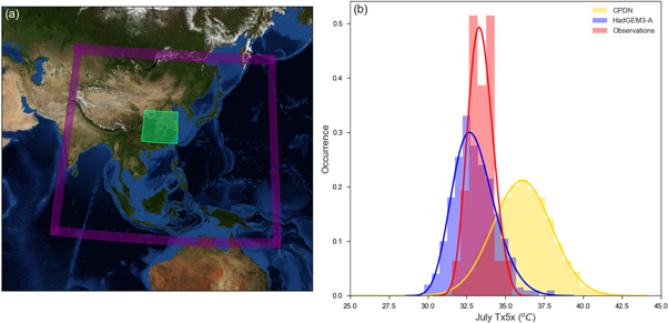
Figure 1. (a) Weather@home East Asia 50 km regional boundary (purple, with shading indicating the regional model sponge layer). The study area for the analysis is shown in green. (b) Distributions of the fractional occurrence of July Tx5x for 1987–2013 from the station data observations (Li et al 2016, red), HadGEM3-GA6 (blue) and weather@home (yellow). For the observations and HadGEM3-GA6 a GEV fit is shown. For weather@home a normal fit is shown.
Download figure:
Standard image High-resolution imageFor the Historical2017 simulations, estimated forcings were used to drive the model with SST and Sea Ice boundary conditions taken from the Operational Sea Surface Temperature and Sea Ice Analysis (OSTIA) dataset (Donlon et al 2011). Sulphur dioxide emissions were taken from the ECLIPSE v5a baseline dataset (Stohl et al 2015, Sparrow et al 2016a, 2016b) and all other forcings were as specified in CMIP5.
For the Natural2017 simulations, pre-industrial forcings were used as specified in CMIP5, with SST changes resulting from anthropogenic forcing (SST deltas, figure S1 is available online at stacks.iop.org/ERL/13/114004/mmedia) from 12 CMIP5 models removed from OSTIA observed values together with a MMM constructed from these 12 models (which is different from MMM-C20C). The SST delta calculation follows the method used in Schaller et al 2016 and were based on the difference between monthly climatologies during 2007–2017 of ensemble mean Historical + RCP4.5 and HistoricalNat CMIP5 simulations. The natural sea ice was taken as the year of maximum extent from the OSTIA observations in both hemispheres independently (as Schaller et al 2016), which corresponds to 1986/1987 in the Northern Hemisphere and 2007/2008 in the Southern Hemisphere. The Natural2017 ensemble is broken down into 12 sub-ensembles based on the individual CMIP5 derived SST driving patterns and the MMM pattern. Each sub-ensemble consists of about 250 members. Freychet et al (2018) used the same model to study heatwaves in China and highlighted its good performance in reproducing summer extreme temperatures (their supplementary figures S2–S4).
Additionally historical simulations (hereafter Historical) were run with OSTIA SST and SIC for the period 1987–2013 to provide a model baseline climatology. As with Historical2017 all other forcings were taken as CMIP5 + RCP4.5 values. Each year was run independently with approximately 190 members per year. Each year started on 1 Dec from 50 simulations that had been spun up for 1 year using conditions from the preceding year. Further initial condition perturbations were applied at the start of each year (to achieve 190 members per year) and run for 13 months. The first month where the model was adjusting to the potential temperature initial condition perturbations was discarded.
The differences in SST used in the weather@home and the HadGEM3-GA6 simulations span a broad range of magnitudes and patterns (figure S1) with broadly positive values everywhere, with some exceptions in the North Pacific and North Atlantic within some models.
3. Analysis methods
Following Chen et al (2018), maximum (Tmax) and minimum (Tmin) near-surface daily air temperature timeseries were computed by area-averaging over the study area (latitude 25-37.5N, longitude 106-122E, green box in figure 1(a)). Both Tx5x and Tn5x datasets were calculated from 5-day running means of Tmax and Tmin, using individual values from each ensemble member. Recall that Tn5x is not a timeseries of maximum Tmin values for July, but rather 5-day Tmin during a coincident period that 5-day Tmax has its maximum July value. This means that in the mathematical sense, Tn5x is not necessarily 'extreme' (but could be if Tn is strongly correlated to Tx) and therefore applying Generalised Extreme Value (GEV) fits to this dataset may not be appropriate.
A GEV fit is applied to the 1987–2013 observational data to determine the return period for the observed 2017 event. For each model, the Historical simulation Tx5x value for this return period is used as the threshold. This is a departure from the Chen et al (2018) methodology, who used the magnitude of the 2017 event as their threshold, and followed that of previous attribution studies (e.g. van Oldenborgh et al 2016, van der Wiel et al 2017 and Otto et al 2018). Both this method and the Chen et al (2018) anomaly threshold method attempt to minimise the effect of temperature bias within the model in slightly different ways. This methodology was chosen over the Chen et al (2018) method to ensure that the same frequency of event was considered in all cases. Error bars for return times show the 5th and 95th percentile computed from 1000 bootstrap (Efron and Tibshirani 1986) samples with replacement. The RR within each model is calculated as the ratio of the probability of exceeding the identified threshold value (in Historical2017) to the probability of exceeding the same threshold value in the Natural2017 simulations. Within this study, we also look at changes in RR over a full range of threshold values corresponding to all return time values in the Historical2017 simulations. The methodology for obtaining uncertainty estimates on RR values is as follows. The probability of exceedance for each threshold value in the full Historical2017 and Natural2017 bootstrap ensembles are calculated and a distribution of possible RR values for that threshold value determined. Uncertainty bounds are taken as the 5%–95% values of this RR distribution. This is repeated for each threshold value.
The Chinese observational data used in this study are homogenized datasets of daily Tmax (and Tmin) with 753 stations in China from 1987–2013 (Li et al 2016). The 2017 record is directly updated from the China Meteorological Data Service Centre. Figure 1(b) shows July Tx5x distributions during 1987–2013 (baseline period) for observations, HadGEM3-GA6 and weather@home. The mean, median and standard deviations for these distributions are given in table S1. HadGEM3-GA6 has a small median cold bias of −0.4 °C but shows a closer agreement to observations than weather@home. The distribution of the weather@home ensemble has a median warm bias of 2.7 °C and is broader than both HadGEM3-GA6 and the observations. The lower end of the tail of the weather@home distribution matches observations although the extreme warm values are over-represented.
July Tx5x is the principal diagnostic used in this study. Thus, within the weather@home ensemble these extreme cases will have a warmer bias, relative to observations, than for HadGEM3-GA6 figure 1(b)). Since all analysis was done in reference to each model's own climatology, the impact of this bias on the outcome of this study is minimised. Within the analysis, the raw output from each model is used to determine the GEV fit parameters, therefore it is necessary to compare the change between Historical2017 and Natural2017 for each model, rather than their absolute values across models, to remove any systematic bias.
4. Results
In this section we present how the risk of a July 2017 type heatwave event changes due to human influences in both the HadGEM3-GA6 and weather@home models. The discrepancy in the magnitude of the RR obtained between the two models is explored and the sensitivity of the result obtained to the particular natural SST pattern used is demonstrated.
4.1. Comparison of return time and RR between models
Figures 2(a), (b) show return times from the Historical, Historical2017 and Natural2017 simulations for Tx5x from both HadGEM3-GA6 and weather@home. As might be expected, the absolute values of the distributions are different between the two models due to different model biases, however all cases show a clear increase in the frequency of Tx5x (and concurrent Tn5x, figure S2) under current climate conditions compared to a world without human influences. The frequency distributions (not shown) from the weather@home simulations are broader than those from HadGEM3-GA6 for Tx5x. Within the same model, the Historical2017 and Natural2017 ensembles have similar distribution widths and analysis is performed with respect to the model climatology to reduce the impact of mean biases. It is important to consider that the increased breadth of the weather@home distributions may result in a lower RR estimate than if the distribution was narrower. Both GEV (solid line) and Normal (dashed line) fits are made to the Tx5x data. In general GEV fits the data well apart from the weather@home Natural2017 simulations, which are better represented by a Normal distribution. The threshold value (corresponding to 87 year return time with a 5%–95% range of 76–102 years, derived from GEV fits to the 1960–2017 observations) is unequaled in the Natural2017 HadGEM3-GA6 ensemble, but becomes approximately a 1 in 50 year event in the Historical2017 ensemble. This return period corresponds to thresholds of 36.7 °C and 40.3 °C for HadGEM3-GA6 and weather@home respectively.

Figure 2. Return times from Historical (yellow), Historical2017 (red), Natural2017 (green) simulations for Tx5x from (a) HadGEM3-GA6 and (b) CPDN weather@home ensemble. Both Normal (dashed black) and GEV (solid black) fits are shown with the exception of 'CPDN Historical' where the GEV fit is poor and omitted from the figure. Risk ratios (y-axis) vs event frequency (x-axis) for 2017 Tx5x for (c) HadGEM3-GA6 (blue) and weather@home (yellow) with 5%–95% uncertainty bounds (d) each of the sub-ensembles (uncertainty bounds omitted for clarity and colors are perceptually uniform from black through purple/red to yellow in increasing order of global mean delta SST).
Download figure:
Standard image High-resolution imageComparing the Historical and Historical2017 ensemble gives an indication of the role of 2017 specific conditions compared to the 1987–2013 period. The 2017 conditions increase the frequency of such events in both models. Using the threshold values above, the RR between Historical2017 and Historical is 3.7 for HadGEM3-GA6 and 2.4 (5%–95% range of 1.8 to 3.3) for weather@home. The event is too rare in the HadGEM3-GA6 Historical ensemble to provide a bootstrap uncertainty estimate on this RR, so the value quoted is based on raw threshold exceedances.
For weather@home (figure 2(b)) Historical and Natural2017 curves are similar (although there is a greater deviation at larger return periods) indicating that the effect of the specific 2017 conditions is similar in magnitude to the effect of human influences alone for the more frequent events. The weather@home RR between Historical2017 and Natural2017 ensembles is 4.8 (5%–95% range of 3.1 to 8.0), which is significantly larger than the increase in risk due to 2017 specific conditions quoted above, i.e. the threshold coincides with separation between the Historical and Natural2017 ensembles. In HadGEM3-GA6 Natural2017 ensemble the 2017 event is unequalled and so no RR is quoted and there is a clear separation between the Historical and Natural2017 curves at all return periods.
Within the weather@home ensemble, 12 different CMIP5 based estimates of Natural SSTs and a MMM pattern were created (see section 2) which were pooled together into the Natural2017 return time curve. If this curve is split into the individual sub-ensembles (table S2, figure S3), then GEV distributions fit most sub-ensembles well. Pooling the results (each with individual GEV fit parameters) changes, as expected, the distribution from a GEV into a Normal distribution. Within figure S3 two model estimates do not fit GEV well (p value <0.5). The return time curves from the individual Natural2017 model estimates have a broad range of distributions (figure S3; Schaller et al 2016), and therefore individually result in a range of different RR.
The median RR of the two models behave differently as a function of return time (figure 2(c)). In general, although different, the agreement between the two models is better at very small return period values than at large values. For HadGEM3-GA6, the RR rapidly increases for return times above three years, whereas a similar transition is not evident in the weather@home results. In both cases, the RR increases for larger return periods, with weather@home decreasing for return periods above 100 years due to sampling uncertainty caused by limited ensemble size. The increase in RR reflects the severity of the event threshold considered. For instance, it might be expected that the rarest events in the Historical2017 ensemble are absent in the Natural2017 ensemble, in which case the RR will be infinity. The magnitude of the differences across a range of return periods is too large to be explained simply by differences in sample size and therefore warrants further investigation.
To investigate this apparently large discrepancy in RR between HadGEM3-GA6 and weather@home, the RR for each of the sub-ensembles of weather@home is computed (figure 2(d)). Considering each natural SST estimate separately yields a diverse range of RR, spanning the RR range seen for both HadGEM3-GA6 and the pooled weather@home results (individual fits derived from GEV parameters for each sub-ensemble are shown in figure S4). This suggests that the RR calculated strongly depends on the construction of the Natural2017 simulations, i.e. the delta SST pattern removed within each sub-ensemble. Figures 2(c), (d) also highlight that when pooling the Natural2017 results together in weather@home, the error estimates derived from bootstrap ensembles show only the sampling error, and fail to capture the added uncertainty due to the different Natural SST patterns used within the ensemble. This is also true when the bootstrap sample size for the pooled Natural2017 weather@home ensemble is limited to the size of the smallest SST ensemble (203 members) and the number of repetitions is increased from 1000–10 000, even though the uncertainty range is increased (figure S5). Therefore, when representing uncertainty in RR derived from the pooled Natural2017 ensembles, it is important to consider the spread in the sub-ensemble results.
4.2. Relationship between RR and global mean SST changes
To understand the source of these differences in RR within the sub-ensembles of the weather@home Natural2017 simulations, the relationship between the GEV fit parameters and the global mean delta SST pattern removed was investigated (figure 3). The GEV shape and scale parameters (figures 3(a), (c)) have poor linear fits as a function of global mean SST delta and show no distinct trend, as evidenced by their R2 and p values. However the GEV location parameter shows a strong inverse relationship with global mean SST delta (figure 3(b)). Natural2017 sub-ensembles with higher GEV location parameters have smaller global mean SST delta and therefore correspond to generally warmer Natural2017 simulations (as might be expected). This relationship translates through to the RR for the simulations (figure 3(d)) where it is the relative change in GEV location parameter between Historical2017 and Natural2017 values that is important. The event frequency of 1 in 5 years was selected to determine the RR values shown. This corresponds to the rarest events that RR can be determined from the model sub-ensembles before results start to deviate substantially from the GEV fit (figure S4). Sub-ensembles with a larger global mean delta SST yield larger and less certain RR as extreme temperatures are rarer in these Natural2017 ensembles. Conceptually, removing a larger delta SST from the observed values will generate a larger difference between the Historical2017 and Natural2017 simulations and so RR further away from 1 would be anticipated. With larger SST deltas and, in this instance, the threshold value corresponding to a position further into the extreme warm tail of the Natural2017 sub-ensemble, greater uncertainty around the RR would be anticipated. The sensitivity of the results to the GEV goodness-of-fit p value shown in table S2 was investigated and found to be robust when screening out results to use only sub-ensembles with p values greater than 0.85 and 0.9 respectively (figures S6 and S7).

Figure 3. July global mean SST differences as a function of Tx5x (a) GEV shape parameter, (b) GEV location parameter, (c) GEV scale parameter and (d) RR for the 1/5 year event. R2, p value and σ (standard error) are given for each linear fit (black). GEV uncertainty estimates are derived from fits to the bootstrap ensemble. Fit lines to the maximum and minimum bounds are denoted by black dashed lines.
Download figure:
Standard image High-resolution image4.3. Sensitivity of RR to regional SST changes
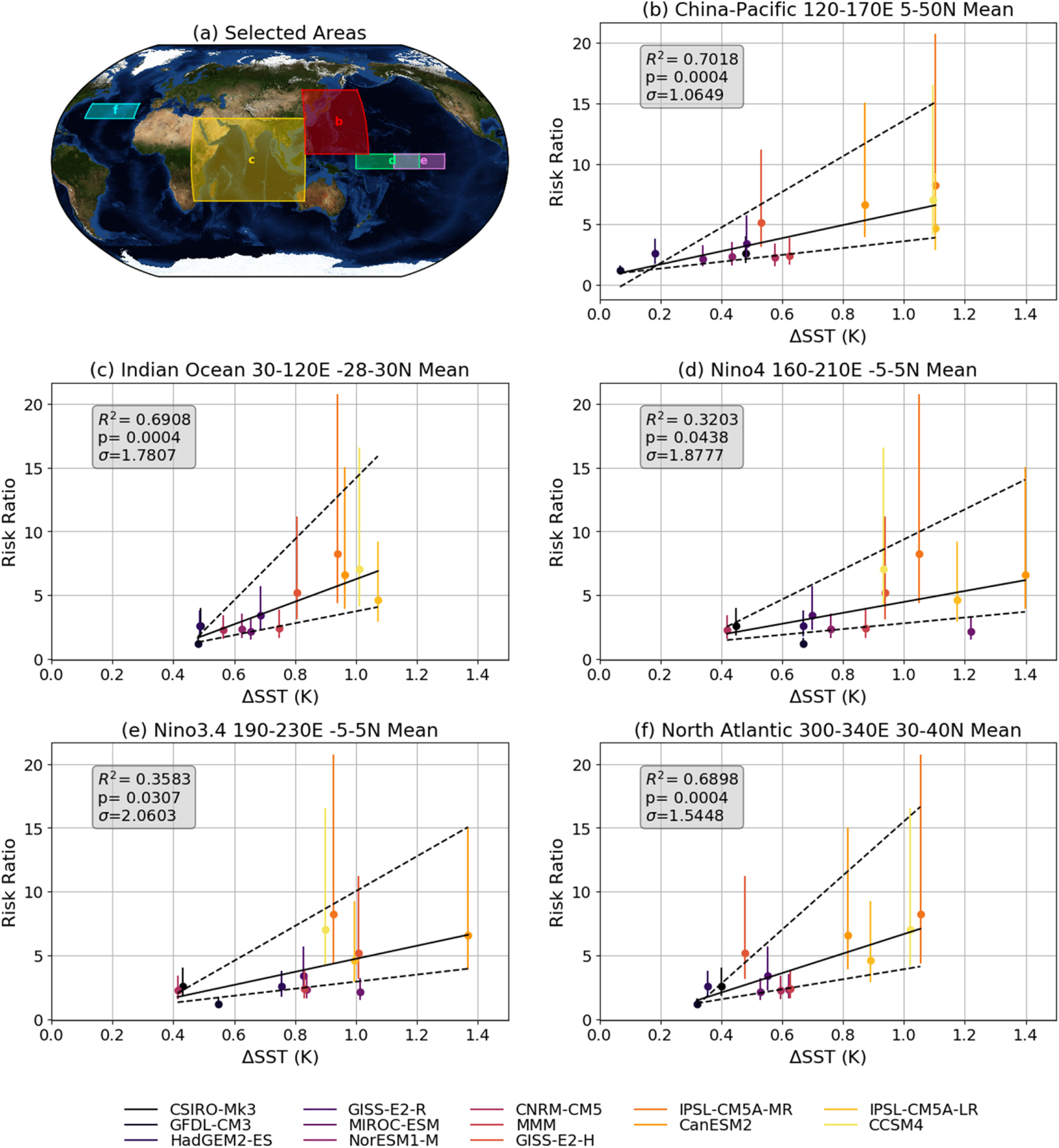
The sensitivity of the relationship between the delta SST and RR (for the 1 in 5 year event) was explored for different ocean regions (figure 4). Five regions were considered (figure 4(a)); 120-170E, 5-50N (China-Pacific); 30-120E, -28-30N (Indian Ocean); 160-210E, -5-5N (Nino4); 190-230E, -5-5N (Nino3.4) and 300-340E, 30-50N (North Atlantic). Although (as seen in figure 3(d)) the global mean delta SST does a good job of broadly capturing the RR differences, individual regions may also be good indicators and correspond to important teleconnection regions for heatwave events in China. As in the global mean case, delta SST in the China-Pacific region (figure 4(b)) are linearly related to changes in RR. The relationship between RR and delta SST appears to be stronger in the Indian Ocean (figure 4(c)) region than in either the Nino4 (figure 4(d)) or Nino3.4 (figure 4(e)) regions. The apparent stronger correlation with Indian Ocean delta SST supports the results in previous studies such as Hu et al (2011), Hu et al (2012), Kosaka et al (2013), who proposed how Indian Ocean variability can impact temperature extremes in China through inducing an anomalous anticyclonic circulation over the western North Pacific and southern China. This is not to say that ENSO is not an important factor in Chinese extreme temperature events as shown previously by Freychet et al (2018). Indeed, studies such as Lau et al (2005) suggest ENSO induced influences on the Indo-Western Pacific SST, and complex interactions between natural variability modes exist within this region, which may be important for Chinese temperature extremes. Li and Ruan (2018) have shown evidence for a North Atlantic-Eurasian teleconnection pattern and suggested that the subtropical North Atlantic Ocean may be influential on Eurasian climate. The dependency of the subtropical North Atlantic difference in SST pattern on RR is explored in figure 4(f), using the region selected in Li and Ruan (2018). Again, there is a broad agreement that the larger the delta SST, the higher the RR. The relationship between RR and delta SST in the North Atlantic better has a steeper gradient than in the Nino3.4 or Nino4 regions and is almost as large as the gradient in the Indian Ocean. The changes in RR from SST changes in both the Indian Ocean and North Atlantic are larger than in the China-Pacific, Nino3.4 or Nino4 regions. The specific role of individual SST regions is undoubtedly complex and warrants further study. Such sensitivities would be better investigated by targeted experiments that isolate SST changes in different regions and consider a range of different lagged responses.

Figure 4. July regional mean SST differences as a function of Tx5x RR. (a) Regions used for plots (b)–(f), (b) China-Pacific (120-170E, 5-50N), (c) Indian Ocean (0-120E, -28-30N), (d) Nino4 region (160-210E, -5-5N), (e) Nino3.4 region (190-230E, -5-5N) and (f) North Atlantic region (300-340E, 30-40N). R2, p value and σ (standard error) are given for each linear fit (black). Fit lines to the maximum and minimum RR bounds are denoted by black dashed lines.
Download figure:
Standard image High-resolution image4.4. Consequence of GEV parameter changes
The change in GEV fit parameters between the Historical2017 and Natural2017 simulations for both models are summarised in figure S8. The change in location parameter in HadGEM3-GA6 is similar in sign and magnitude to the equivalent change in weather@home (with all sub-ensembles indicating a reduction in this parameter between Historical2017 and Natural2017 conditions). Both the shape and scale parameters show divergent results between the two models with a broad range of values (of both signs) across the weather@home sub-ensembles particularly for the shape parameter. To further explore the role of each GEV parameter on the RR, the impact of changing each GEV parameter in turn was explored (figure 5). RR as a function of event frequency were computed based on GEV fit parameters. One (light dashed line), two (dotted line) or all three (dark solid line) GEV fit parameters (for both HadGEM3-GA6 and weather@home) were changed systematically from the parameter values in the Natural2017 ensembles to the parameter values in the Historical2017 ensembles to form a hypothetical distribution to compare with the Natural2017 distribution when calculating the RR. In each of the three panels, the labels 'Constant ΔLocation', 'Constant ΔShape' and 'Constant ΔScale' refer to the fact that the specified parameter always takes the Historical2017 value in the hypothetical ensemble and so maintains the same difference compared with the Natural2017 in the RR calculation in all lines shown.

Figure 5. RR as a function of return time, obtained from comparing hypothetical distributions using one or more of Historical2017 GEV fit parameters relative to Natural2017 GEV fit parameters. HadGEM3-GA6 is shown in blue and pooled CPDN weather@home in yellow. The RR derived for lines within each subpanels are based on hypothetical distributions where the GEV parameter denoted in the title takes on the Historical2017 value. The effect of allowing only a single parameter to take on Historical2017 values is denoted by the light dashed line at the edge of the shaded region and the effect of allowing all three GEV parameters to take on Historical2017 values is shown by the dark solid line at the edge of the shaded region. The arrows indicate the direction of change in RR resulting from allowing a single parameter change between distributions to allowing all GEV parameters to change. Dotted lines show the effect of relative changes in both the location and shape parameters (panel a) , shape and scale parameters (panel b), and scale and location parameters (panel c). The black solid line represents zero change in risk.
Download figure:
Standard image High-resolution imageWhen only the location parameter is changed from Natural2017 to Historical2017 while the shape and scale parameters are held at their Natural2017 values in the hypothetical distribution (figure 5(a), light dashed line), the HadGEM3-GA6 and weather@home results are much closer than when all parameters are changed to Historical2017 values (dark solid line). This suggests that the effect of changing the location parameter alone (from the value under Natural2017 to Historical2017) is similar between HadGEM3-GA6 and combined sub-ensembles of weather@home (consistent with figure S8). Therefore it is the differences in the relative change of the shape and scale parameters that contribute strongly to the divergence of the two model results (as indicated by the diverging arrows in figures 5(a) and S8). Changing both the location and shape parameters (dotted line) shows that differences in shape parameter contribute most strongly to the diverging results, with a small contribution from differences in the scale parameter. This is supported by changing the shape parameter alone (figure 5(b), light dashed lines) where the two models show a marked divergence at return times greater than ∼10 years. Additionally, when both the scale and location parameters differ between the hypothetical and Natural2017 distribution (figure 5(c), dotted lines), profiles are similar indicating the largest divergence arises from the relative difference in the shape parameter between the hypothetical and Natural2017 ensemble. Marked differences emerge when the scale parameter alone is changed (figure 5(c), light dashed lines), but only for the very rarest events. For return periods greater than 50 years the RR is dominated by relative differences in the shape parameter whilst relative differences in the location parameter dominate at lower return periods.
Changes in the GEV shape parameter relate to how extreme the tail of the distribution is. As shown in figures 2 and S3, combining the different naturalised SST patterns in weather@home makes the distribution 'less extreme' so that a normal distribution fits better than GEV. It also has the effect of 'averaging' in some way the range of location parameters from each sub-ensemble into a single value (figures 2(c), (d)). The difference between GEV and normal distributions relate to the tail, principally affecting the shape parameter. This may account for the differences in RR with event frequency seen in the two models particularly for the return periods greater than 50 years.
As noted earlier, GEV fits to the Historical2017 weather@home ensemble are poor, therefore a similar analysis was performed using the location and scale parameter from a Normal fit to the data (figure 6). The effect of changing the location parameter alone (light dashed line) between the hypothetical ensemble and Natural2017 results in RR at all return times that are closer than when both the location and scale parameters change (dark solid line). Relative differences in the scale parameter (i.e. the width of the distribution) between Natural2017 and Historical2017 ensembles acts in opposite directions for HadGEM3-GA6 and weather@home in a similar manner to the GEV fit results. This is further exemplified by allowing the scale parameter alone to change between the distributions (dotted lines). The effect of changing scale parameter on the RR is larger for the rarer (and more extreme) events as might be expected. This would imply that for weather@home the Historical2017 ensemble is narrower than the Natural2017 ensemble, whereas in HadGEM3-GA6 the Historical2017 ensemble is broader than the Natural2017 ensemble. This would be consistent with a broader range of possible Natural2017 states being available in the weather@home ensemble as a result of including a wider range of SST patterns compared to HadGEM3-GA6. The earlier assertion that differences between Normal and GEV distributions relate to changes in the tail, principally affecting the shape parameter, and therefore translate to RR changes for return periods greater than 50 years is further supported by comparing figures 5 and 6. This is particularly evident in the HadGEM3-GA6 ensemble.

Figure 6. RR as a function of return time, obtained from comparing hypothetical distributions using one or more of Historical2017 Normal fit parameters relative to Natural2017 Normal fit parameters. HadGEM3-GA6 is shown in blue and pooled CPDN weather@home in yellow. Light dashed lines show when only the location parameter differs from Natural2017 values in the hypothetical ensemble. Similarly, dotted lines show when only the scale parameter differs from Natural2017 values and dark solid lines show when both location and scale parameters take on Natural2017 values. The arrows indicate the direction of change in RR resulting from allowing only the location parameter to change and allowing both location and scale parameters to change. The black line represents zero change in risk.
Download figure:
Standard image High-resolution image
5. Discussion and conclusion
During July 2017 a record-breaking heatwave event occurred in Central Eastern China, severely impacting public health, agriculture and infrastructure (China Climate Bulletin 2017). This study assessed the role of human activity in changing the likelihood of this event by using two different Met Office Hadley Centre models, each run under two climate scenarios representing the world with and without human influences. Historical simulations from both models show the specific conditions of 2017 provided an increased likelihood for July Tx5x compared to the recent period (1987–2013) of 2.4 (5%–95% range of 1.8 to 3.3) for weather@home with the HadGEM3-GA6 raw value of 3.7 lying beyond the upper end of this range. Both models show that July 2017-like heatwave events in China have become more likely due to human activity, however the precise magnitude of the increase in risk depends on the model used and SST patterns used to construct the naturalised simulations. The event is unequaled in the HadGEM3-GA6 Natural2017 ensemble (differing from Chen et al (2018) because of methodology and baseline climatology used) and corresponds to a RR of 4.8 (5%–95% range of 3.1 to 8.0) in weather@home. The larger the global mean delta SST pattern removed in the Natural2017 ensemble, the larger the change in GEV location parameter (relative to Historical2017) which in turn leads to a higher (and more uncertain) RR.
A simple exploration of the dependency of the RR on different geographic regions of SST has been explored based on relevant regions noted in the literature. These initial findings show that although all regions broadly show a dependence on the delta SST pattern removed, the SST difference over the Indian Ocean and North Atlantic gives a larger change in risk than the China-Pacific, Nino4 or Nino3.4 regions. These results suggest that further investigation of the impact of SST, in different regions and at different lags, on Central Eastern China heatwave events would be of interest.
The effect on the RR of changing one, two or all three GEV parameters from Historical2017 to Natural2017 values in both models was explored and the result shows the event corresponds to more than a simple shift in the distribution. When just the location or both the location and scale parameters were changed, the RR obtained between the two models were comparable. Changes to the shape parameter were found to cause the largest divergence between the two model results and contribute most strongly to the RR for return periods greater than ∼50 years. Changes in the location parameter dominate at shorter return periods, with the July 2017 China heatwave sitting on the transition point between these dominating parameters. The shape parameter is related to how extreme the distribution of Tx5x is. By pooling results from each naturalised SST pattern into a single ensemble, this is in effect altering the distribution from GEV to normal and can therefore partly explain the differences in RR seen between the two models for longer return periods.
The concurrent Tn5x results (figure S3) show that the event was not only extreme in terms of Tx5x in July but also in Tn5x, with the RR of the event being larger at all return times than seen for Tx5x. High night-time temperatures such as this can be especially important when considering the public health implications of extreme heat events as no respite from the elevated temperature is available (Weisskopf et al 2002, Meehl et al 2004).
The results of this study highlight the importance of incorporating a plausible range of different natural SST patterns within attribution studies to properly represent this dependency and to better sample the uncertainty. Also, given this relationship, observational uncertainty for SSTs used to drive historical simulations should also be represented. Pooling results derived from a range of different natural SST patterns results in a 'mean' of the range of responses from individual estimates. However, if pooled results are quoted, the uncertainty estimates derived from bootstrapping are likely an under-representation of the true uncertainty and therefore RR uncertainty should be derived from the response of individual SST estimates.
Acknowledgments
This work and its contributors (S S, F T, N F, F L, B D, S T, D W) were supported by the UK-China Research & Innovation Partnership Fund through the Met Office Climate Science for Service Partnership (CSSP) China as part of the Newton Fund. WC were supported by National Natural Science Foundation of China No. 41675078. The authors would like to thank Karsten Haustein for his assistance with generating delta SSTs and Friederike Otto for useful discussions and the comments and suggestions provided by two anonymous reviewers. We would like to thank the Met Office Hadley Centre PRECIS team for their technical and scientific support for the development and application of weather@home. Finally, we would like to thank all of the volunteers who have donated their computing time to climateprediction.net and weather@home.